using Turing, AlgebraOfGraphics, CairoMakie, DataFrames
using AlgebraOfGraphics:density
using DataFrames:stack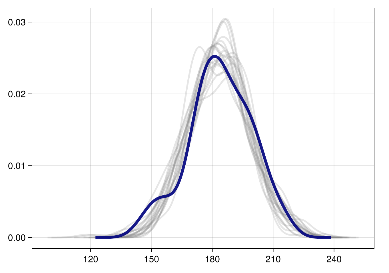
Bayes in Julia
For the past few weeks I’ve been trying out Julia as a tool for Bayesian stats. There’s a lot to like about the language, most of which has been covered elsewhere. It’s intuitive, it’s fast, and it’s fun. Granted, it’s also a young ecosystem, so there may be fewer resources available depending on your area of interest. Fortunately, probabilistic programming and Bayesian inference is a space that’s seen plenty of growth recently.
As a mostly-R person, I’ve been using brms and rstan for some time now, so I was curious to try out Turing.jl (here) for my Bayesian workflow. Don’t get me wrong, the Stan-based ecosystem is wonderful, and I’d say brms is the friendliest tool to get your feet wet with Bayesian modeling. Also, the amount of tutorials, guides, and general content available is vast (special shoutout to Solomon Kurz’s translation of Statistical Rethinking). And Stan (accessed through whichever interface works best for you) still tops the charts in terms of reliability, speed, and documentation.
But brms (and every other tool that uses lm or lme4-based syntax) also abstracts away details that I feel are important if we want to better understand how Bayesian inference works behind the scenes. Instead, Turing (very much like raw Stan, or McElreath’s rethinking package in R) makes you spell out every part of your model. But it’s also written entirely in Julia, which makes it incredibly interoperable (and more accessible than raw Stan).
For example, you can include tools from any other Julia libraries or use different samplers if you want.
A model of height
Ok, let’s get started. For this, you’ll need the following packages. Note that I’m also calling a couple of functions because they share names with functions in other packages. This allows me to call density without having to specify that I want the AlgebraOfGraphics implementation.
Let’s start with a very simple toy model, based on a Statistical Rethinking example. We have a bunch of height measurements and we’re trying to infer the mean (mu) and standard deviation (sigma) of our population.
As you can see below, models in Turing are just functions, preceded by the @model macro. Here, height_mean is the name of the model.
Aside, if you don’t know what a Julia macro is, head here.
@model function height_mean(; n = 1)
    mu ~ Normal(175, 20)
    sigma ~ Exponential(1)
    y ~ filldist(Normal(mu, sigma), n)
end
height_mean (generic function with 2 methods)That’s it. We set our prior for the mean (mu) to 175cm because it’s a reasonable average height, and our prior for sigma (the standard deviation) to a fairly harmless exponential distribution (though note there are better priors for scale parameters). I’ve added n as a parameter because it will come in handy for prior predictive checks and other things.
A couple of notes about the likelihood. The filldist syntax creates an n-length vector of Normal(mu, sigma) distributions, which gives us a performance boost over loops. But we can still use loops. The code above is equivalent to this:
@model function height_mean(; n = 1)
    mu ~ Normal(175, 20)
    sigma ~ Exponential(1)
    for i in 1:n
      y[i] ~ Normal(mu, sigma)
    end
end
One thing I really appreciate about Turing is how easy it is to use for a full Bayesian workflow including prior predictive checks, model iteration, model checking, or posterior predictive checks, for example.
Let’s do some prior predictive checks to see whether our model is producing reasonable results before seeing the actual data.
To do that, we can just use call the rand function (which generates samples from a given generator) on our model to get our mu, sigma and y, straight from the prior.
One thing that’s lovely about Julia is how modular it is. Note that if I want to take samples from a Normal distribution I can just create a distribution object and use the
rand function to sample it. There’s no need for a specific sampling function for every distribution family.rand(height_mean())(mu = 165.49691935056015, sigma = 0.3013854035355912, y = [165.35444024123953])Let’s do this a 1000 times and visualize our results. Note that throughout this blog post we’ll use Makie.jl and AlgebraOfGraphics.jl (which is built on top of Makie) to plot our analyses and results.
To learn more about
Makie.jl, head here.y_prior = vcat([rand(height_mean()).y for i in 1:1000]...)
hist(y_prior)
Looks pretty reasonable! Very few people are over 220 cm (or under 120 cm) tall, so this makes sense overall. Note that there’s actually another way to do prior predictive checks. We can just use the sample function that we’ll use later on, but specifying that we want the samples to come from the prior.
y_prior_chn = sample(height_mean(), Prior(), 1_000);

df = DataFrame(y_prior_chn)

hist(df[:,"y[1]"])
We get very similar results.
Conditioning and sampling
Next, let’s generate our fake data to see whether our model can recover our parameters. Let’s assume our sample of heights comes from a place where the average person is quite tall (e.g. the Netherlands). Let’s have our real mu be 185cm, and our sigma be 15. Once again, we can use the rand function to get 100 samples.
y_fake = rand(Normal(185, 15), 100)

first(y_fake, 5)
5-element Vector{Float64}:
179.14497444673466
169.31526276323365
167.08122537276944
179.9675689163041
167.5129143676516Now, let’s condition our model on the fake data we generated. To do this in Turing, we can just use |, as shown below. We can then sample from the conditioned model using our sampler of choice.
Here we’re using the no U-turn sampler (NUTS), and we’re running it for 1000 iterations and 2 chains. MCMCThreads() allows us to run chains in parallel if that’s needed.
cond_model = height_mean(; n = length(y_fake)) | (;y = y_fake);

m1_chn = sample(cond_model, NUTS(), MCMCThreads(),  1_000, 2);
Now we can go ahead and see whether our model recovers the real parameters.
Model checking
Let’s use the summarystats function to take a look at our results.
summarystats(m1_chn)Summary Statistics parameters mean std naive_se mcse ess rhat ⋯ Symbol Float64 Float64 Float64 Float64 Float64 Float64 ⋯ mu 183.3720 1.5016 0.0336 0.0344 1880.3006 0.9996 ⋯ sigma 15.2470 0.9675 0.0216 0.0203 2181.6638 0.9998 ⋯ 1 column omitted
That’s not bad at all! Let’s plot the parameters using AlgebraOfGraphics. Note that the StatsPlot (based on Plots.jl) provides off-the-shelf to work with chain objects, but I personally prefer the Makie family. It’s straightforward and highly customizable.
df_chn = DataFrame(m1_chn)

plt = data(df_chn) * mapping(:iteration, [:mu :sigma])
plt *= mapping(color = :chain => nonnumeric, row = dims(2)) * visual(Lines, alpha = 0.7)

draw(plt)
Our chains have mixed well. Let’s plot the actual parameters.
plt = data(df_chn) * mapping([:mu, :sigma])
plt *= mapping(col = dims(1)) * histogram(bins = 20, datalimits = extrema)

draw(plt; facet = (; linkxaxes = :none))
Note that we could have also reshaped the dataframe into long format. However, AlgebraOfGraphics has good support for wide data, so it’ll work either way.
chn_long = stack(df_chn, [:mu, :sigma])

plt = data(chn_long) * mapping(:value)
plt *= mapping(col = :variable) * histogram(bins=20, datalimits = extrema)

# draw the plot
draw(plt, facet = (linkxaxes = :minimal,))
Posterior predictive checks
Finally, some posterior predictive checks. Let’s generate 100 draws from the model. We then stack the dataframe (or pivot_longer if you’re in R) to make it easier to work with.
# get the predictions
predictions = predict(height_mean(; n = 100), m1_chn)

# stack the dataframe
df_long = stack(DataFrame(predictions), 3:102)

# keep just 20 ddraws
df_long = subset(df_long, :iteration => ByRow(x-> x<=20))
First, let’s do a density overlay plot. As a reminder, this plots the original data (shown in dark blue) overlayed with a number of posterior predictive samples (showing in light grey). We can use this to assess whether our generative model is capturing the features of the real data.
# plot the posterior predictive samples
plt = data(df_long) * mapping(:value)
plt *=  mapping(group = :iteration => nonnumeric)
plt *= visual(Density, color = (:white, 0),
    strokecolor = (:grey, 0.2),
    strokewidth = 3)

# plot the original data
plt2 = data((;y = y_fake)) * mapping(:y) * visual(Density, color = (:white, 0),
    strokecolor = (:navy, 0.9),
    strokewidth = 5)

both = (plt + plt2)

# draw both layers
draw(both)
That’s pretty good! Which makes sense, because it’s a very simple model, and we generated the data ourselves.
Let’s also do some histograms, comparing the distribution of the original data with 14 draws from the posterior (why 14? it’s a nice number and it’ll fit in a 3x5 grid including the original data).
# keep just 14 draws
df_hist = subset(df_long, :iteration => ByRow(x-> x<=14))


plt = data(df_hist) * mapping(:value, layout = :iteration => nonnumeric)

plt *= histogram(bins=20) * visual(color = :grey, alpha=0.4)


plt2 = data((;y= y_fake)) * mapping(:y)
plt2 *= histogram(bins=20) * visual(color = :navy, alpha = 0.7)
Layer(AlgebraOfGraphics.Visual(Any, {:color = :navy, :alpha = 0.7}) ∘ AlgebraOfGraphics.HistogramAnalysis{MakieCore.Automatic, Int64}(MakieCore.Automatic(), 20, :left, :none), (y = [179.14497444673466, 169.31526276323365, 167.08122537276944, 179.9675689163041, 167.5129143676516, 173.14049255371256, 194.02095323245283, 160.73859222151324, 172.82434970656556, 186.67500788914083 … 194.60925937976683, 170.6911063030617, 169.51659051941783, 196.88120605204483, 199.24394114055528, 160.70712226008547, 172.354374931714, 176.39932231465602, 180.11454493489586, 186.45320095995854],), Any[:y], {})Now let’s see whether we can manage to plot both the original data and the model predictions.
ncol = 5
nrow = 3

fg = draw(plt; palettes = (layout = vec([(j, i) for i in 1:ncol, j in 1:nrow])[2:end],),
facet = (linkxaxes = :none,),
axis = (width = 550, height = 350))

draw!(fg.figure[1, 1], plt2)

fg
And that’s it! Next time we’ll look at some other Turing models and dig deeper into how we can use Makie/AlgebraOfGraphics for our Bayesian workflow.