data {
int<lower=2> K; // number of categories
int<lower=0> N; // number of observations
int<lower=1> D; // number of predictors
int<lower=0,upper=K> y[N]; // response variable
matrix[N, D] x; // design matrix
}
parameters {
vector[D] beta; // predictors for ordered logistic part (e.g. likert scale)
ordered[K-1] c; // number of thresholds for ordered logistic
real alpha_p; // intercept for proportion of non-response
vector[D] beta_p; // predictors for proportion of non-response
}
model {
// model
vector[N] mu;
vector[N] eta;
for (n in 1:N) {
mu[n] = alpha_p + x[n] * beta_p;
eta[n] = x[n] * beta;
// assume non-response coded as 0
if (y[n] == 0)
// predict non-response using a bernoulli
target += bernoulli_logit_lpmf(1| mu[n]);
else
// otherwise use ordered logistic
target += bernoulli_logit_lpmf(0| mu[n]) + ordered_logistic_lpmf(y[n]| eta[n], c);
}
}
generated quantities {
// generate samples
vector[N] yrep;
for (n in 1:N) {
if (bernoulli_rng(inv_logit(alpha_p + x[n] * beta_p)) == 1)
yrep[n] = 0;
else
yrep[n] = ordered_logistic_rng(x[n] * beta, c);
}
}
Surveys contain all types of data: categorical (What country were you born in?), numeric (How many people live in your household, including you?), text (If Other, please specify:), and, most importantly for this blog post, ordinal data (How happy do you feel today?). And ordinal data, as I’ve mentioned in the past, can be tricky to deal with.
Ordinal data is often treated as metric. This is not great, because it can lead to faulty inference, including detecting effects that aren’t really there, missing real effects, or even finding an effect of the opposite sign.
That’s why we have ordinal models. Now, using a metric model for your ordinal data does not always lead to catastrophe. Often it’s completely fine. But, like Kruschke and Liddell say, the way to check whether your metric treatment of the data is appropriate is to double check by fitting an ordinal model. And, at that point, why not just use the ordinal model?
Surveys, surveys
Surveys often contain plenty of ordinal questions with a limited number of options, because they’re useful! They’re easy to understand, and often less cognitively costly than open-ended questions or questions that ask for numeric input.
For questions like these, you have a whole family of models to choose from. If you’re interested, Paul Bürkner and Matti Vuorre have an excellent tutorial paper centered around models from the psychology literature. Two of the most popular choices are the ordered logit and ordered probit.
But consider a question like this one:
Tell me how much confidence you have in German Chancellor Angela Merkel to do the right thing regarding world affairs – a lot of confidence, some confidence, not too much confidence, or no confidence at all.
Note that this survey was administered in the United States! This is a classic Likert-scale question, but (by virtue of asking about a foreign leader) it’s also one that is likely to prompt a fair amount of “don’t know” responses, because many respondents may genuinely not know who Angela Merkel is, or they don’t have a formed opinion on whether they trust her.
Here’s the breakdown of responses, provided by Pew (and accessible here):
library(gt)
library(tidyverse)
library(hrbrthemes)
library(scales)
library(gghighlight)


responses <- c("Don't know / refused",
             "A lot of confidence",
             "Some confidence",
             "Not too much confidence",
             "No confidence at all")

results <- tibble(Response = responses,
             Proportion = c(0.12, 0.16, 0.40, 0.14, 0.18)) %>%
  mutate(Response = factor(Response, levels = responses))

gt(results) %>%
tab_header(title = md("How much confidence do you have in **Angela Merkel**?"))| How much confidence do you have in Angela Merkel? | |
|---|---|
| Response | Proportion |
| Don't know / refused | 0.12 |
| A lot of confidence | 0.16 |
| Some confidence | 0.40 |
| Not too much confidence | 0.14 |
| No confidence at all | 0.18 |
Let’s show this in a plot. Clearly Americans don’t love Angela Merkel as much as other countries do, but we’ll soon see that this varies depending on who you ask!
results %>%
  ggplot(aes(y = Response,
             x = Proportion)) +
  geom_col(fill = "#00A08A") +
  theme_ipsum_ps() +
  labs(title = "Americans' confidence in Angela Merkel",
       y = NULL,
       x = NULL) +
  theme(plot.title.position = "plot") +
  scale_x_percent() +
  gghighlight(Response == "Don't know / refused")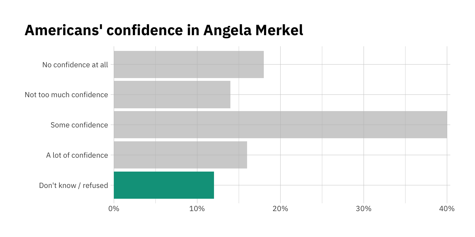
Back to our ‘don’t know’ data. Around 12% of respondents said they didn’t know, or refused to answer. That’s a lot!
Analyzing the data
Ok, so what do we do with these responses if we want to predict confidence in Merkel according to a set of variables of interest? The simple (and unfortunate) answer is that most of the time this data is just removed and treated as missing.
Missing data is routinely mistreated. It is often discarded, which is both inefficient (since we’re throwing away data) and dangerous (since missingness may have originated in ways that affect our analysis!). It is also replaced with means, 0s. We know all of these options are far from ideal. There are better ways to treat missing data in both response and predictor variables. A more appropriate way to do it is to ask ourselves how the missingness originated, include our missingness in a DAG, and engage in multiple imputation (here’s a recent example by Solomon Kurz using brms).
Don’t know isn’t missing
But it feels a bit strange to impute ‘don’t knows’ because it’s not missing data. The respondent did answer, after all.
Effectively, we have a problem: A chunk of our responses follow an ordinal logic (those who do decide to give an answer), and one of the options does not (don’t know). That means we can’t really use a simple ordinal model, because the ‘don’t know’ option doesn’t follow a clear ordering and there’s no obvious place to put it.
One potential (and simple) way to deal with this is to assume that this is categorical data, and just use a multinomial likelihood (as, for example, when you ask people what their favorite color is). But this choice is not ideal because we’re throwing away information We know that the Likert part of your response is ordinal, but we’re telling your model to treat it as though it were not.
So what can I do? In principle, I want to be able to model my ordinal responses and my don’t knows separately, because they potentially respond to different data generating processes. This is one of the reasons why mixture models exist. For example, zero-inflated Poisson regression (ZIP) is used to model counts with an excess of zeros. Similarly, zero-one-inflated Beta regression can be used to model proportions that include 0s and 1s, or even visual slider data, as Matti Vuorre did here.
Mixtures to the rescue
I ended up putting together a simple Stan mixture model that incorporates a Bernoulli likelihood to model the probability of non-response, and the ordinal part is handled by an ordinal logistic likelihood.
To keep it simple, we will assume all ‘don’t knows’ are coded as 0, and all ordinal responses start at \(k=1\).
The full likelihood looks something like this:
\[ \text{ZiOrderedLogistic}(k~|~\eta,c, \theta) = \left\{ \begin{array}{ll} \theta & \text{if } k = 0, \\[4pt] (1-\theta) \cdot \text{OrderedLogistic}(k~|~\eta,c) & \text{if } 1 \leq k < K \end{array} \right. \]
Ok, let’s build the model. I’ve looked through some of the Stan forums and resources, but please let me know if you see anything catastrophically wrong.
We’ll start with the ordered logistic model provided in the Stan manual, and then add a Bernoulli likelihood with an if-else statement, following the example of the zero-inflated Poisson model found here.
Note that in our basic model we have the same predictors for each part of the model, but there’s a separate vector to store the parameter for each. Our vector beta_p will contain the coefficients of predictors for the probability of non-response, and our vector beta will contain the predictors for the regular ordinal. Finally, we added a generated quantities chunk to include samples for post-processing.
Let’s load the data and libraries we’ll need. You can find the clean Merkel confidence data on this Github repo, as well as the Stan model used.
Note that in this example we are using the same predictors for non-response and confidence ratings, but this isn’t necessary. The model can be easily tweaked to have separate predictors (or no predictors at all if we’re just interested in overall probability of non-response).
To keep it simple, we’ll use four dummy variables based on the Pew Data. The four dummies we’ll include in the model are: party affiliation (Democratic-leaning), education (4 year post-secondary degree, or more), race (identifies as non-white), and income (over $75,000 in annual income).
library(readr)
library(dplyr)
library(rstan)
library(bayesplot)
library(tidybayes)
library(patchwork)

csv_url <- "https://raw.githubusercontent.com/octmedina/zi-ordinal/main/merkel_data.csv"

data <- read_csv(csv_url)

D <- 4 # number of predictors
N <- length(data$confid_merkel) # number of observations
y <- data$confid_merkel # response variable
x <- matrix(c(data$party, # predictors
              data$edu,
              data$race,
              data$income),
            nrow = N, ncol = D)
K <- length(unique(data$confid_merkel)) - 1 # number of ordinal levels (0 doesn't count)


stan_data <- list(
  N = N,
  K = K,
  y = y,
  x = x,
  D = D)
Note that in our data, lower scores are better, and 0’s are non-responses. Keep this in mind for our coefficient plots! Here’s the breakdown:
| Coded values | |
|---|---|
| Response | Score |
| Don't know / refused | 0 |
| A lot of confidence | 1 |
| Some confidence | 2 |
| Not too much confidence | 3 |
| No confidence at all | 4 |
Let’s fit the model using rstan.
stan_url <- "https://raw.githubusercontent.com/octmedina/zi-ordinal/main/zi-ordinal-model.stan"

fit_merkel <- stan(file = stan_url,
                   data = stan_data,
                   chains = 4,
                   cores = 4,
                   iter = 2000)
Looking at the results
The model fits fine, with no divergent transitions or mixing issues. We can check whether the chains have mixed using mcmc_trace from the bayesplot package.
mcmc_trace(fit_merkel, pars= c("beta[1]", "alpha_p", "beta_p[1]", "c[1]") )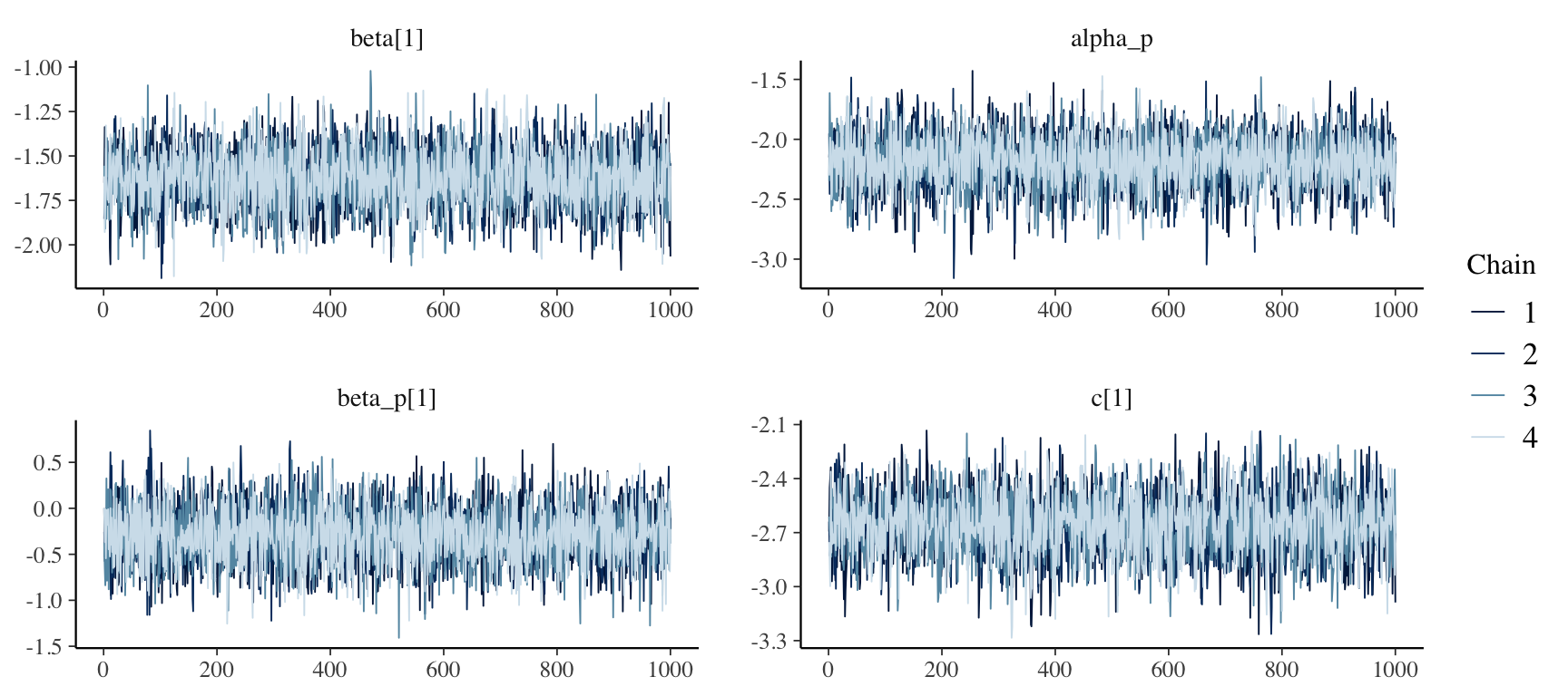
The chains seem to have mixed well. Let’s look at the model summary for our parameters of interest:
print(fit_merkel, pars= c("beta", "c", "alpha_p", "beta_p"))Inference for Stan model: zi-ordinal-model.
4 chains, each with iter=2000; warmup=1000; thin=1;
post-warmup draws per chain=1000, total post-warmup draws=4000.
mean se_mean sd 2.5% 25% 50% 75% 97.5% n_eff Rhat
beta[1] -1.63 0 0.16 -1.95 -1.73 -1.63 -1.52 -1.31 4231 1
beta[2] -0.68 0 0.16 -1.00 -0.79 -0.68 -0.58 -0.37 5506 1
beta[3] 0.70 0 0.21 0.28 0.56 0.70 0.84 1.11 7105 1
beta[4] -0.02 0 0.15 -0.32 -0.12 -0.02 0.08 0.28 5574 1
c[1] -2.66 0 0.17 -3.00 -2.77 -2.66 -2.54 -2.32 3391 1
c[2] -0.15 0 0.13 -0.40 -0.24 -0.14 -0.06 0.11 5213 1
c[3] 0.84 0 0.14 0.57 0.74 0.84 0.93 1.11 5558 1
alpha_p -2.19 0 0.23 -2.65 -2.34 -2.19 -2.03 -1.77 5112 1
beta_p[1] -0.28 0 0.31 -0.89 -0.49 -0.28 -0.07 0.32 5121 1
beta_p[2] -0.69 0 0.34 -1.35 -0.91 -0.68 -0.46 -0.04 5612 1
beta_p[3] 0.68 0 0.36 -0.03 0.46 0.69 0.92 1.40 5593 1
beta_p[4] -0.40 0 0.32 -1.02 -0.62 -0.39 -0.17 0.20 6057 1
Samples were drawn using NUTS(diag_e) at Tue Nov 30 21:11:09 2021.
For each parameter, n_eff is a crude measure of effective sample size,
and Rhat is the potential scale reduction factor on split chains (at
convergence, Rhat=1).Ok that’s quite interesting! Our predictor variables seem to affect the ordinal ratings and the probability of non-response in different ways. This is much more informative than what we would’ve gotten had we just looked at the complete cases and deleted the ‘don’t knows’.
But let’s plot the coefficients and get our variable names back, since right now it’s not very intuitive to follow. Recall that we had 4 predictors: leans Democratic, has a college degree or more, identifies as non-white, and has an annual income of over $75k.
Here’s the coefficients plot. We used tidybayes get the posterior samples and then plot their distributions. Note that the effect sizes are in log-odds!
merkel_draws <- fit_merkel %>%
  spread_draws(beta[condition], beta_p[condition])


merkel_draws %>%
  ggplot(aes(y = fct_rev(factor(condition,
                                levels = c(1, 2, 4, 3),
                                labels = c("Democrat", "College degree", "Over $75k", "Non-White"))),
             x = beta)) +
  stat_halfeye(.width = c(.90, .5)) +
  theme_ipsum_pub() +
  labs(y = NULL,
       title = "Effect on Confidence in Merkel - Ordinal",
       subtitle = "Negative coefficients imply higher levels of confidence",
       x = "Effect Size (Log-Odds)") +
  theme(plot.title.position = "plot")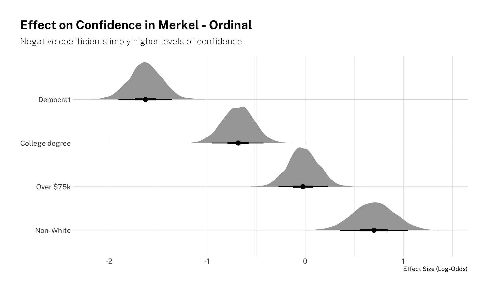
Identifying as a Democrat is the biggest predictor of respondents’ confidence in Merkel. Democrats consistently show more confidence in the (now former) German chancellor. The same is true (though to a lesser extent) by voters with a college degree. Being wealthier does not seem to be a strong predictor either way, while identifying as non-white is predictive of worse ratings.
Now, let’s look at the effect sizes on the probability of non-response. Note that being college-educated and white makes respondents more likely to provide a response. Democrats and the high-income are also less prone to fall in the “don’t know / refuse” category, though the estimated coefficients are noisier.
merkel_draws %>%
  ggplot(aes(y = fct_rev(factor(condition,
                                levels = c(1, 2, 4, 3),
                                labels = c("Democrat", "College degree", "Over $75k", "Non-White"))),
             x = beta_p)) +
  stat_halfeye(.width = c(.90, .5)) +
  theme_ipsum_pub() +
  labs(title = "Effect on Non-Response",
       subtitle = "Negative coefficients imply more non-response",
       x = "Effect Size (Log-Odds)",
       y = NULL) +
  theme(plot.title.position = "plot")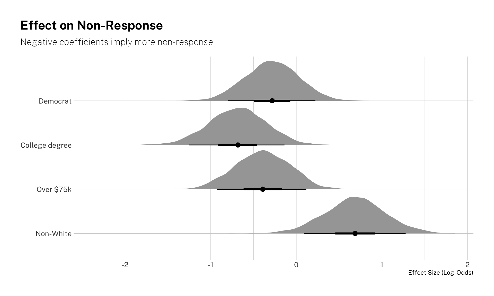
Some more visualization
How big are these effects? Our coefficients are shown in log-odds. This is not the most intuitive scale, so let’s show the difference in predicted non-response for some demographic groups. Let’s pick some that are predicted to have high non-response, and some that are predicted to have low non-response.
merkel_nonresponse <- fit_merkel %>%
  spread_draws(alpha_p, beta_p[..])


merkel_nonresponse <- merkel_nonresponse %>%
  mutate(`White, Republican, No College, <75k` = alpha_p,
         `Non-White, Republican, No College, <75k` = alpha_p + beta_p.3,
         `White, Republican, College, >75k` = alpha_p + beta_p.2 + beta_p.4,
         `Non-White, Democrat, College, >75k` = alpha_p + beta_p.1 + beta_p.2 + beta_p.3 +  beta_p.4,
          `White, Democrat, College, >75k` = alpha_p + beta_p.1 + beta_p.2 + beta_p.4) %>%
  mutate(across(9:13, ~plogis(.)))


merkel_nonresponse_long <- merkel_nonresponse %>%
  pivot_longer(9:13, values_to = "non_response", names_to = "condition")

factor_levels <- merkel_nonresponse_long %>%
  group_by(condition) %>%
  summarize(median = median(non_response)) %>%
  arrange(-median)

merkel_nonresponse_long %>%
  mutate(condition = factor(condition, levels = factor_levels$condition)) %>%
  ggplot(aes(y = condition, x = non_response)) +
  stat_halfeye(.width = c(.90, .5)) +
  theme_ipsum_pub() +
  labs(title = "Predicted Non-Response by Demographic",
       x = NULL,
       y = NULL) +
  theme(plot.title.position = "plot") +
  scale_x_percent()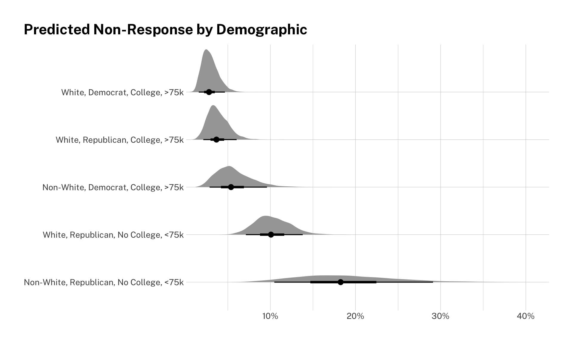
Look at that! The probability of non-response varies quite a bit. Note that the large confidence intervals for non-whites is due to the small sample in the survey.
Probabilities
We can also look at the expected probability of falling in each level of the ordinal scale. This is very simple to do in brms and rstanarm (more on this in a later blog post), but since we’re doing pure rstan we’ll have to do some extra work. First, we need to convert the log-odds into probabilities of falling into each bucket.
Our probability mass function for a zero-inflated ordered logistic with K levels looks like this:
\[ \text{Pr}(k~|~\eta,c, \mu) = \left\{ \begin{array}{ll} \text{logit}^{-1}(\mu) & \text{if } k = 0, \\[4pt] 1 - \text{logit}^{-1}(\eta - c_1) & \text{if } k = 1, \\[4pt] \text{logit}^{-1}(\eta - c_{k-1}) - \text{logit}^{-1}(\eta - c_{k}) & \text{if } 1 < k < K, \text{and} \\[4pt] \text{logit}^{-1}(\eta - c_{K-1}) - 0 & \text{if } k = K. \end{array} \right. \]
So we’ll need to come up with a function to recreate it. Thank you to Solomon Kurz, Henrik Singmann, and Mattan Ben-Shachar for this discussion, which was extremely useful for this purpose. It turns out that this is not as bad as it seems :
return_prob <- function(mu, eta, c) {
  c <- c[[1]]
  p_zi <- plogis(mu) # inverse-logit
  n_thresh <- length(c) # get number of thresholds

  # create the probabilities for all the categories
  p_total <- cbind(p_zi, (1-p_zi)*(1-plogis(eta-c[1])))

  for (i in 2:n_thresh) {
    p_total <- cbind(p_total, (1-p_zi)*(plogis(eta-c[i-1])-plogis(eta-c[i])))
  }

  p_total <- cbind(p_total, (1-p_zi)*(plogis(eta-c[n_thresh])))

  p_total
}
Let’s make sure that this works:
return_prob(-3, -2.5, list(c(-3.5, -1, -0.1))) p_zi
[1,] 0.04742587 0.2561866 0.5226137 0.09454568 0.07922816It works! Let’s go ahead and calculate the predicted probabilities for each of our options.
merkel_all <- fit_merkel %>%
spread_draws(alpha_p, beta_p[..], beta[..]) %>%
janitor::clean_names()
merkel_c <- fit_merkel %>%
spread_draws(c[i]) %>%
janitor::clean_names() %>%
group_by(chain, iteration, draw) %>%
summarize(c = list(c))
t <- merkel_all %>%
mutate(mu_1 = alpha_p,
eta_1 = 0,
mu_2 = alpha_p + beta_p_3,
eta_2 = beta_3,
mu_3 = alpha_p + beta_p_2 + beta_p_4,
eta_3 = beta_2 + beta_4,
mu_4 = alpha_p + beta_p_1 + beta_p_2 + beta_p_3 + beta_p_4,
eta_4 = beta_p_1 + beta_p_2 + beta_p_3 + beta_p_4,
mu_5 = alpha_p + beta_p_1 + beta_p_2 + beta_p_4,
eta_5 = beta_p_1 + beta_p_2 + beta_p_4)
prob_1 <- return_prob(t$mu_1, t$eta_1, merkel_c$c) %>%
as_tibble() %>%
mutate(condition = "White, Republican, No College, <75k")
prob_2 <- return_prob(t$mu_2, t$eta_2, merkel_c$c) %>%
as_tibble() %>%
mutate(condition = "Non-White, Republican, No College, <75k")
prob_3 <- return_prob(t$mu_3, t$eta_3, merkel_c$c) %>%
as_tibble() %>%
mutate(condition = "White, Republican, College, >75k")
prob_4 <- return_prob(t$mu_4, t$eta_4, merkel_c$c) %>%
as_tibble() %>%
mutate(condition = "Non-White, Democrat, College, >75k")
prob_5 <- return_prob(t$mu_5, t$eta_5, merkel_c$c) %>%
as_tibble() %>%
mutate(condition = "White, Democrat, College, >75k")
joint <- bind_rows(prob_1, prob_2, prob_3, prob_4, prob_5) %>%
mutate(condition = factor(condition))
my_labels <- c("Don't know",
"A lot of confidence",
"Some confidence",
"Not too much confidence",
"No confidence at all")
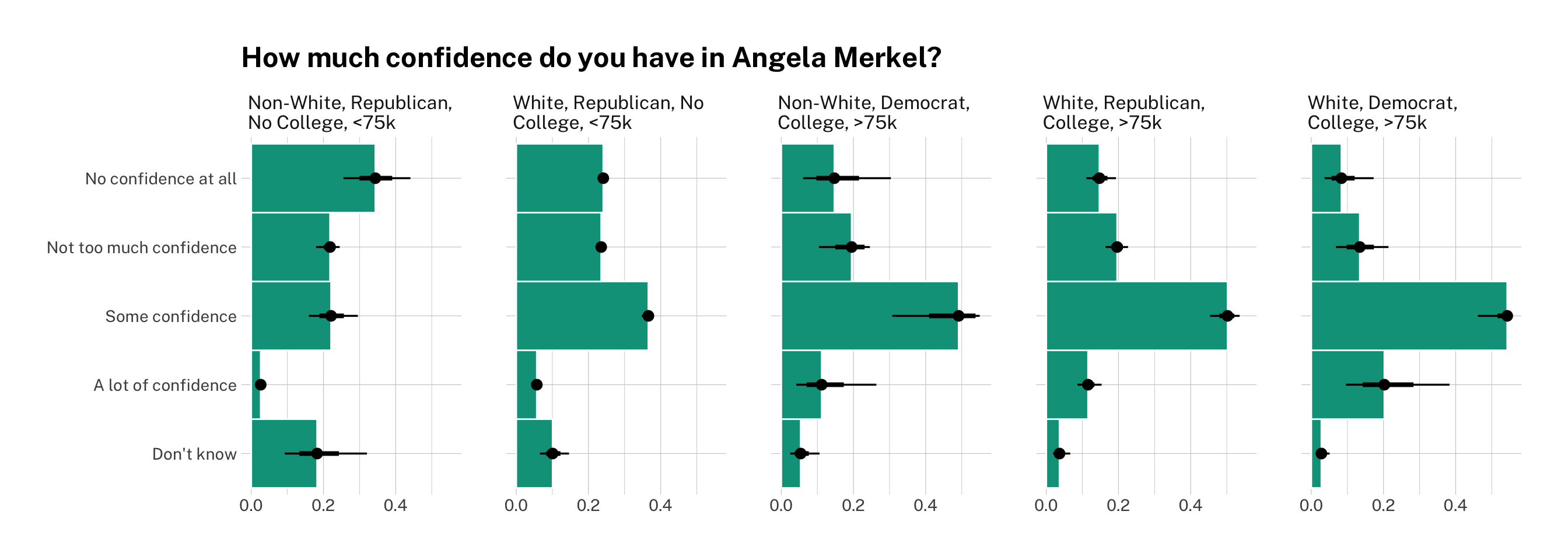
names(joint)[1:5] <- my_labels joint %>%
pivot_longer(1:5) %>%
mutate(name = factor(name, levels = my_labels),
condition = factor(condition, levels = factor_levels$condition)) %>%
ggplot(aes(y = name, x = value)) +
facet_grid(~condition, labeller = label_wrap_gen(width = 25, multi_line = TRUE)) +
stat_summary(fun = median, geom = "bar", fill = "#00A08A", width = 1, color = "white") +
stat_pointinterval() +
theme_ipsum_pub() +
labs(y = NULL,
x = NULL,
title = "How much confidence do you have in Angela Merkel?")
Now we have the full predicted probability distributions for each of our categories and groups of interest! Once again, you can see that Republicans, non-white respondents, and respondents with no college degree are less likely to have confidence in Angela Merkel and the latter two are also more likely to say say they don’t know or would rather not respond.
Democrats, on the other hands, are much more likely to rate the Chancellor highly. Being wealthy is associated with a greater probability of response, but does not seem to affect views on Merkel either way.
Posterior predictive checks
Finally, since we’ve generated samples in our generated quantities block, we can do some posterior predictive checks to see how well our model predicts the data:
stan_yrep <- rstan::extract(fit_merkel)$yrep

ppc_bars(y = data$confid_merkel,
         yrep = stan_yrep)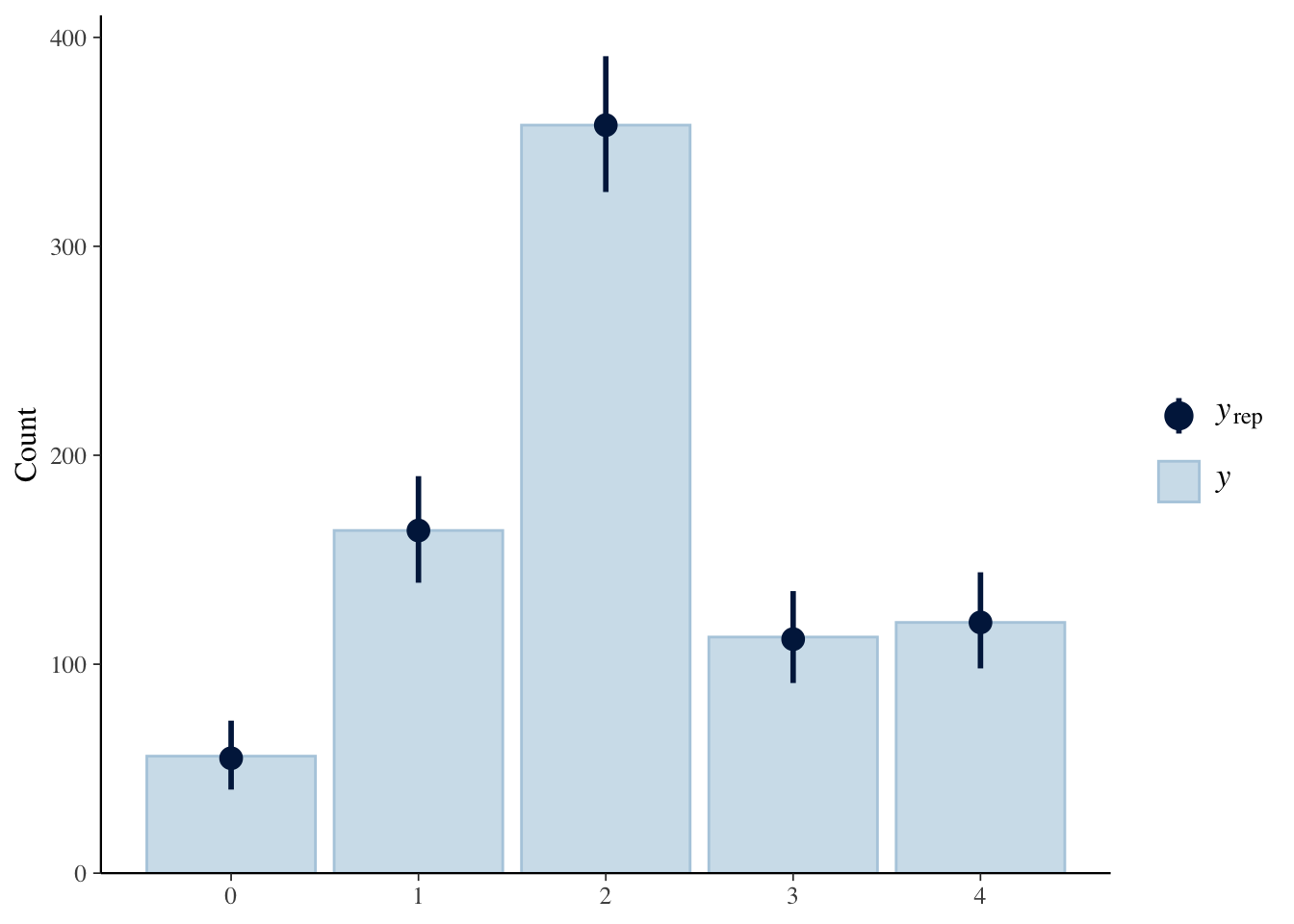
Bingo! The model accurately represents our existing data. Let’s look at some of the groups of interest. For example, education and party.
p1 <- ppc_bars_grouped(y = data$confid_merkel,
                 yrep = stan_yrep, group = as.factor(data$edu)) +
  labs(title = "Education (College or more)")


p2 <- ppc_bars_grouped(y = data$confid_merkel,
                 yrep = stan_yrep, group = as.factor(data$party)) +
  labs(title = "Party (Democrat)")


p1 + p2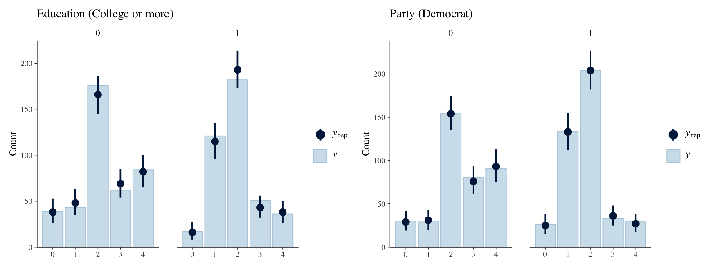
Not bad at all. All of the predicted counts fall under the 95% credible intervals, which is a good sign.
So what?
Was this all worth it? Who knows, but I would say it’s a better way of trying to deal with ‘don’t know’ responses than restricting your sample to complete cases. Often, non-response is correlated with plenty of variables of interest, so using a model that incorporates predictors of this non-response allows us to be aware of whose views we may be missing, and may prove useful when analyzing survey data.
Extensions
The next step is translating this into brms. Thanks to Paul Bürkner’s vignette, this is more straightforward than it may seem. But that’s for a future blog post.